Conditional formatting
This can be found on the Home > Style > Conditional Formatting.
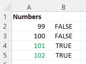
Whenever you want to want to use a formula, I found it easier to do this trick. Create the formula next to the column you want to apply the formatting. In the case below, I want to check if the value is greater than 100 (=A2>100, =A2>100 etc)
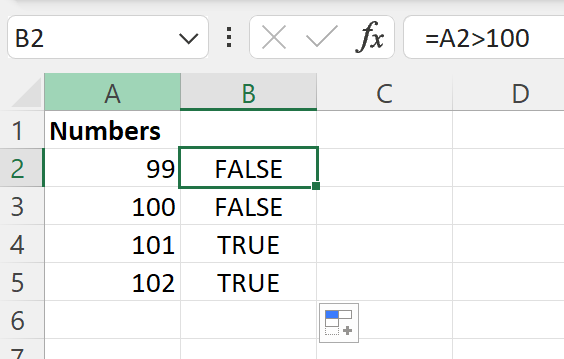
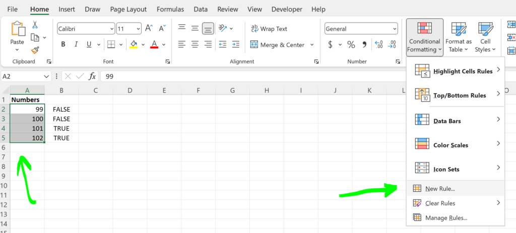
As we can see the formula works just fine as we get the values TRUE and FALSE. Now it’s time to apply it to the Numbers column and set the colour GREEN if TRUE. Select the range, go to Conditional Formatting and select New Rule…
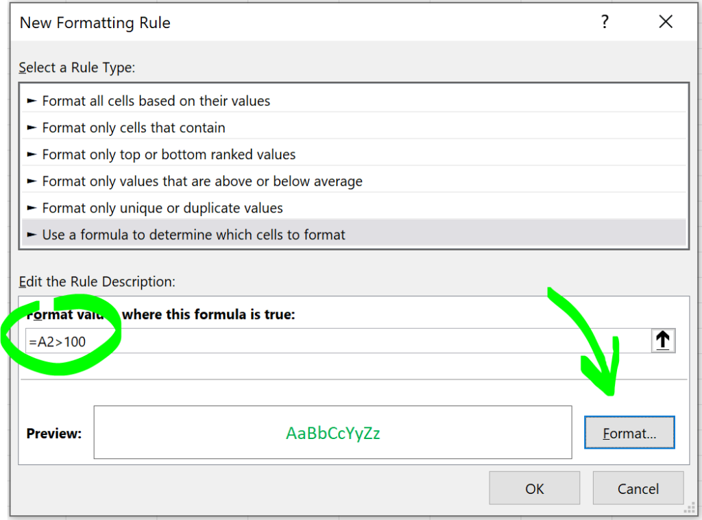
Enter the Formula and set the format.
The results:
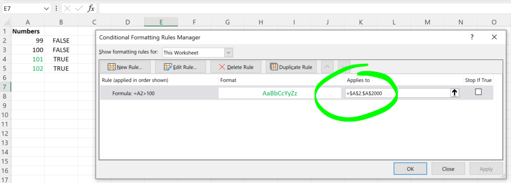
To extend the formula for all the rows I’ve modified the Applies to value to =$A$2:$A$2000
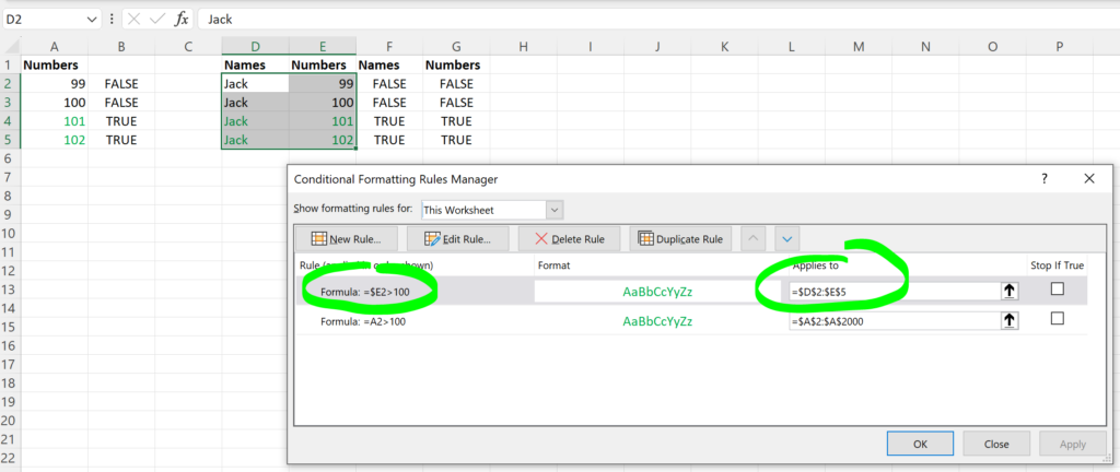
To format more columns with the same formula use the same logic. By using the dollar sign I was able to lock the column (E) which I want to use in my formula.
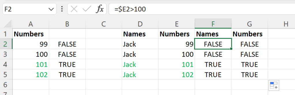
Then I applied the formula next to my table and as you can see F and G match in values. Now I can go an add this as Conditional Formatting.
Dollar Symbol ($) in an Absolute Reference
A particularly useful and common symbol used in Excel is the dollar sign within a formula. Note that this does not indicate currency; rather, it’s used to fix a cell address in place in order that a single cell can be used repetitively in multiple formulas by copying formulas between cells.
=C6*$C$3
By adding a dollar sign ($) in front of the column header (C) and the row header (3), when copying the formula down to Rows 7–15 in the example below, the first part of the formula (e.g., C6) changes according to the row it is copied down to while the second part of the formula ($C$3) stays static always enabling the formula to refer to the value stored in cell C3.